Maching Learning In Production Infrastructure
In the previous post, we looked at the components of Machine Learning Ops at a high level and briefly touched on each stage of the life cycle. With this in mind, we can now look at the finer processes of a machine learning infrastructure solution and begin to explore the tooling and technologies used in their curation.
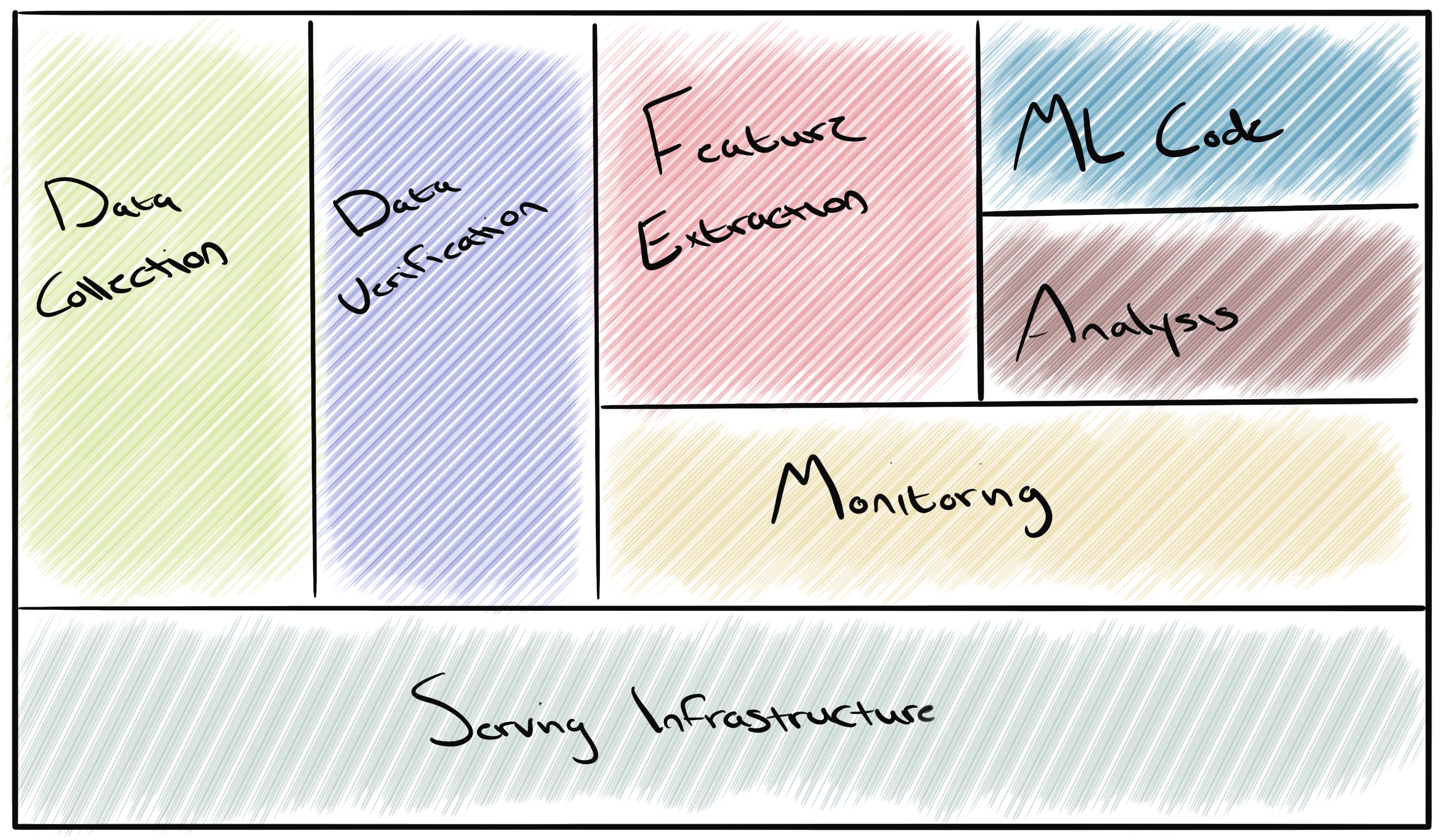
Looking at the image below, you’ll notice that the machine learning code is only a small portion of the overall solution. The bulk of tooling within machine learning infrastructure exists to support the capture, integration and monitoring of data ingested and produced by the model. The quality and accuracy of model produced data is largely dependant on the quality of data ingested as well as the measures which have been put in place to either enrich or verify the data. The smallest of changes in a data set can compound over time and ultimately lead to quite a sizeable, negative impact to model performance. Most of us will be familiar with the term GIGO ( Garbage In Garbage Out ) and this remains an important concept to keep in consideration when building machine learning solutions.
The sections below will provide some insight into each of the main objectives of the infrastructure components that a machine learning solution is comprised of.
Data Collection
The data collection step focuses on the collection of data from a number of chosen data sources. Depending on what you are training your model to do, data sources can be text based forums for language learning, social media sites or generic websites for images, or youtube videos to collect audio or video samples. The amount of data and the frequency at which it is collected is all dependant on a number of factors and is something that is often finely tuned as the solution evolves.
There are a number of ways which data for machine learning can be collected and collection methodologies will differ depending on what works best. A few example sources are:
Open Source Datasets
Web Scraping
- Price extraction from e-commerce sites.
- Scraping of plain text from text based forums or websites.
Manual Data Collection
- Raw data from physical or virtualised sensors.
- Survery or forum responses.
Data Verification
Once data collection has been completed, it is then important to verify the data to ensure it is both accurate and up to date before it is consumed by the remaining components. We can imagine the data verification step as a gate at which all data must satisfy a set of requirements before being allowed to continue on its journey. As an example, we may want to remove duplicate entries from a data set to avoid inflating the weight of a particular value which could lead to its significance being misrepresented and ultimately contribute to model inaccuracy.
We may also wish to ensure that the data conforms to a specific schema prior to it’s continuation. For example if we have parameters that are expecting a specific number format, we should ensure that all numerical values provided by this feature are of the same format and within an expected range.
Feature Selection
Feature selection aims to finely tune collected data and reduce noise by removing variables which are adding little to zero value to the performance of the model. Whilst it’s often beneficial to have a large volume of data for training models, it’s important to identify which parts of this data are contributing to model performance and which are not. Having large, complex data sets consisting of a lot of noise will only slow down the model training process and result in a slower model overall.
For example, imagine we are training a model to predict the sale price of houses in a given year and we are presented with a dataset that consists of the below features.
| Sale Price | Overall Condition | Year Built | Total Sq Foot | Property Slope |
|---|---|---|---|---|
| 150,000 | 1 | 1975 | 2000 | 0.1 |
| 140,000 | 0.8 | 1988 | 1800 | 0.2 |
| 200,000 | 0.9 | 2000 | 2400 | 0.1 |
| 480,000 | 1 | 2010 | 3500 | 0.5 |
| 85,000 | 0.6 | 1991 | 1100 | 0.2 |
| 155,000 | 0.5 | 2001 | 1500 | 0.3 |
| 170,000 | 0.8 | 2001 | 1600 | 0.6 |
| 230,000 | 0.7 | 1996 | 1900 | 0.1 |
Looking at the above, we may determine that the Property Slope feature may not be as impactful to model performance due to a lack of enough variance to make an impactful change. Therefore, we should remove this from consideration leaving the data set to be used for training as below:
| Sale Price | Overall Condition | Year Built | Total Sq Foot |
|---|---|---|---|
| 150,000 | 1 | 1975 | 2000 |
| 140,000 | 0.8 | 1988 | 1800 |
| 200,000 | 0.9 | 2000 | 2400 |
| 480,000 | 1 | 2010 | 3500 |
| 85,000 | 0.6 | 1991 | 1100 |
| 155,000 | 0.5 | 2001 | 1500 |
| 170,000 | 0.8 | 2001 | 1600 |
| 230,000 | 0.7 | 1996 | 1900 |
Pipelining and Configuration
The pipelining step of a machine learning solution is not greatly indifferent from that of more common infrastructure solutions. The aim is to integrate the various infrastructure components that houses the model and supporting technologies and where possible, ensure the repeatable aspects of the workflow have been automated. Like any CI/CD, we need to understand what our data sources are, where they are housed and understand how this data will traverse the various components.
In addition to data, the pipeline will be responsible for the deployment of serving infrastructure as well as the management and delivery of the model code itself.
Source Code
Depending on their purpose, machine learning projects will most likely involve multiple source code repositories, each consisting of a different language depending on the nature of the overall solution. However, for the purpose of this post and simplicity, we’ll consider that the source code consists of code bases that are responsible for the preparation of data and the development of the model.
There are a number languages used to train models and their selection is largely dependant on preference as well as a few other factors. However, some of the common languages accompanied by a few of the most commonly used learning and data libraries within each are:
Python
R
JavaScript
C++
Resource Management
With resource management, we can again draw on a number of similarities from the management of resources in more common platform solutions. At the core, we’re looking to strike a balance between minimising the costs and maximising the value produced by the solution. However, machine learning requires a considerably greater amount of computational power over common cloud computing applications. This is because for machine learning models to be efficient, they require the ability to process multiple computations simultaneously. Whilst it is possible to train and deliver models using only CPU equipped instances, if you’re dealing with deep learning applications or neural networks it is incredibly beneficial to employ instances equipped with either GPUs or TPUs due to their large number of cores and matrix multiplication optimisation.
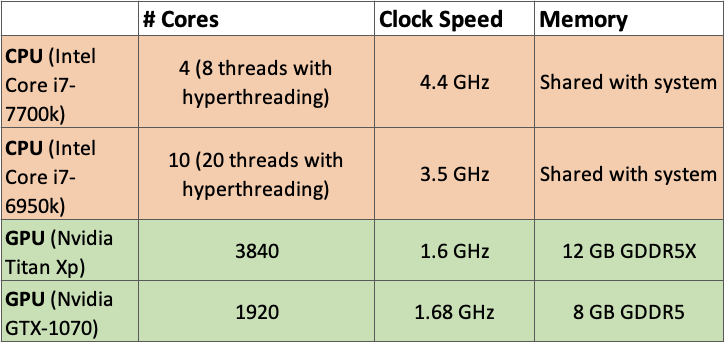
GPU or TPU equipped instances can get incredibly expensive and their justification must be weighed against a few other factors. For example, how quickly do we need to be able to ingest and enrich new data, train our model and then deliver the newly produced model to a production environment? If this needs to be a short period of time, then we will most likely need a GPU or TPU equipped instance to speed up this delivery time. If this is not the case and we can afford a longer amount of time between the delivery of new models, then it may be more cost effective to only utilise hardware equipped with less powerful hardware and accept the longer training time. Additionally, costs for services providing functionality such as storage can be greatly inflated when delivering a machine learning solution. The greater the size of the model and the data set it requires, the greater the cost of storage.
Monitoring
Aside from the usual performance metrics, monitoring machine learning infrastructure in production environments should place a large focus on testing the integrity and performance of the model itself. There are a number of ways this can be done and we’ll cover these in depth in a further post but for now, some of the most common methods are as below:
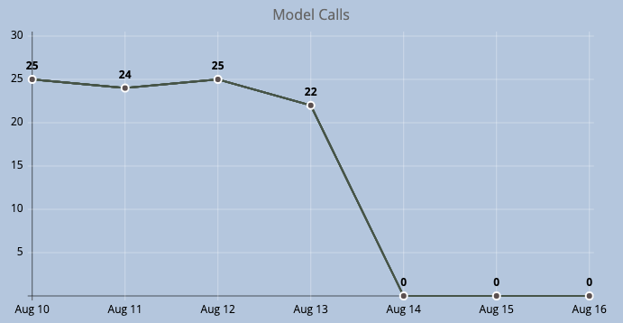
Model Call Monitoring
If we treat our model in a similar fashion to that of a public endpoint. We monitor the amount of calls which have been made to the model and the percentage of these calls which have returned a response successfully. If the number of calls being made to the model drops to 0, or begins to display anomalies when compared to normal usage patterns, we can deduct there is an issue.
We can also employ metrics such as response time. How long is the model taking to return a response? If this begins to exceed predetermined or acceptable thresholds then again we can assume something is not functioning as intended.
Feature Change and Schema Monitoring
Within a machine learning solution, it’s important that we’re able to maintain the integrity of the data at each step of the process to allow us to identify any potential issues. One method to do this is to monitor the data schema itself for any intended or accidental changes. The aim here is to be alerted to any drop, addition or change of the current data set features. We’ll also be able to then compare the accuracy metrics of the model against the various points at which the schema / feature set has changed and determine the impact the change had on the accuracy of the model.
Additionally, monitoring the values of the features is important to ensure the contained data is both correct and usable. For example, if we are expecting numerical values from a specific feature but upon querying character based values are returned instead, we should have monitoring in place to identify this discrepancy.
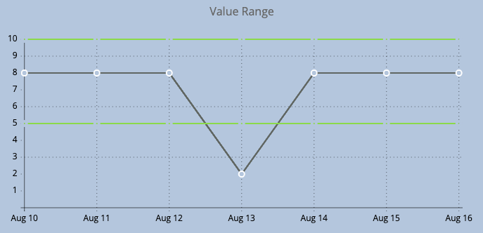
It may also be the case that the feature values are of the intended type but the values themselves are falling outside of the expected range. For example, a specific feature may be expected to return a numerical value between the range of 5 and 10 but when queried, numbers outside of this range are being returned. We should again be able to represent this graphically and have alerting in place to identify this.
Missing Data
As with unintended data types and incorrect values, we need to have the capability to identify missing values in data streams that are being ingested by the model. This being said, monitoring for missing values and any abnormality within the data set should be done with a certain level of fault tolerance. The level of tolerance applied should of course be determined by the level of impact which abnormal values will have on the performance of the model.
Whilst the above focused on the base metrics that we can expect when monitoring a machine learning solution, there are a number of additional caveats which it is best to prepare for, two examples are Model Decay and Data Drift which we’ll cover in depth in a further post.